Exercises

This exercise is from book An Introduction to Statistical Learning with R.

1. (a) Better. A more flexible method will obtain a better estimation with large sample size. (b) Worse. A more flexible approach will cause over-fitting when the number of predictors is extremely large and the number of observations is small. (c) Better. With more degree of freedom, a flexible approach will obtain a better fit. (d) Worse. Flexible approaches will fit to the noises and increase the variance of error terms.

2. (a) Regression. We are interested in inference. Quantitative output of CEO salary. $n$: the top of 500 firms in the US. $p$: profit, number of employees, industry. (b) Classification. We are interested in prediction. Predict the new product's success or failure. $n$: 20 similar products. $p$: price charged, marketing budget, competition price, and ten other variables. (c) Regression. We are interested in prediction. Quantitative output of the % change in the dollar. $n$: All weekly data of 2012. $p$: the % change in the US market, the % change in the British market, the % change in the German market.

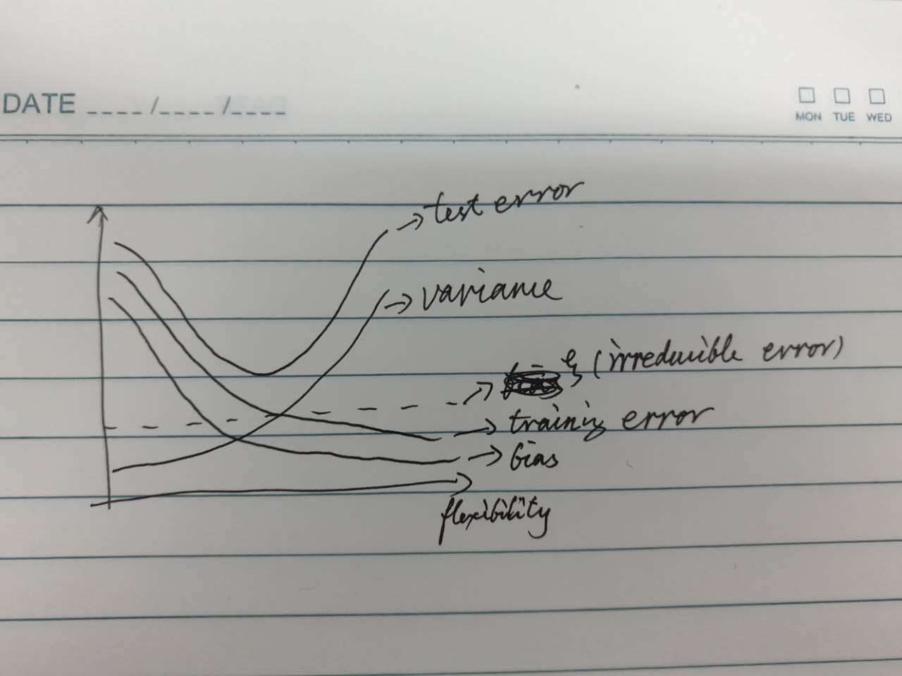
3. (a) (b) bias: Generally, more flexible methods result in less bias. variance: The variance of error terms will increase with the increasing of flexibility of methods, since they will attempt to fit the noises. $\epsilon$(irreducible error): The irreducible error is the limit of test error, the under-bound of test error. training error: It likes bias in some way. But on the other hand, the lower training error may induce higher variance. test error: It is the sum of bias, variance and $\epsilon$, when the level of flexibility is too high, may cause over-fitting.

4. Well, there are many examples, and alright, I'm a little lazy now.

5. The biggest advantage of a very flexible model is it can estimate a better $\hat{f}$ than less flexible models. The biggest disadvantage of a very flexible model is it may easily cause over-fit. When we wanna a prediction, the higher flexible methods will be preferred, and when we wanna a inference, the less flexible methods will be preferred.

6. The parametric methods assume a form of $f$, but non-parametric methods don't assume a particular functional form of $f$. The advantages of parametric methods are they can simplify the model of $f$ to a fewer parameters, and don't require a large number of observations. The disadvantages of parametric methods are they may also cause over-fit if using a more complex model.

7. (a) 3.000000 2.000000 3.162278 2.236068 1.414214 2.236068 (b) Green, since the nearest distance is 1.414214, and that observation is Green. (c) Could be green or red, cause the top 3 nearest distances when K=3 are 1.414214, 2, 2.236068. The observations are #2 #4 #5 #6, and the color could be {'green', 'green', 'red'} or {'red', 'red', 'green'} cause we can choose #4 or #6 randomly. (d) Small. A small value of K is more flexible for non-linear decision boundary.

8. see below

(a)

college <- read.csv('data', header=T)

(b)

rownames(college) <- college[,1] fix(college) college <- college[,-1] fix(college)

(c)

summary(college) pairs(college[,1:10]) plot(college$Private, college$Outstate) Elite <- rep("No", nrow(college)) Elite[college$Top10perc > 50]="Yes" Elite <- as.factor(Elite) college <- data.frame(college, Elite) summary(college$Elite) plot(college$Elite, college$Outstate) par(mfrow=c(2,2)) hist(College$Apps) hist(College$Accept, col=3) hist(College$Enroll, col='cyan', breaks=10) hist(College$Top10perc, breaks=10)

1. see below

(a)

sapply(Auto, class)

(b)

sapply(Auto[, 1:7], range)

(c)

sapply(Auto[, 1:7], mean) sapply(Auto[, 1:7], sd)

(d)

newAuto <- Auto[-c(10, 85),] sapply(newAuto[1:7], range) sapply(newAuto[1:7], mean) sapply(newAuto[1:7], sd)

(e)

pairs(Auto)

(f)

Not each predictor is useful, most variables have relationship with mpg, but the variable 'name' should not be used. It has no relationship with mpg, and may cause over-fit.

1. see below

(a)

dim(Boston)

(b)

pairs(Boston)

(c)

see section (b)

(d)

par(mfrow=c(3,1)) hist(Boston$crime[Bosten$crime > 1], breaks=10) hist(Boston$tax, breaks=30) hist(Boston$ptratio, breaks=30)

(e)

length(Boston$chas[Boston$chas==1])

(f)

median(Boston$ptratio)

(g)

Boston$zn[Boston$medv\==min(Boston$medv)] Boston[Boston$medv\==min(Boston$medv),] sapply(Boston, range)

(h)

length(Boston$rm[Boston$rm > 7]) length(Boston$rm[Boston$rm > 8]) summary(Boston[Boston$rm > 8, ]) summary(Boston)